Before we proceed, you might be tempted to ask (or maybe not), there are already gazillion articles on this. What’s different here? Anyhow, in how many different ways can one even present the same 16-page literature?

In this article my aim is to bridge the theoretical aspect that most text on the cerfnet very nicely present, but take it a step further to connect with the real world implementation of the said text.

Bridging idea with action. That’s what this post tries to offer.

Yet, we should start with the theoretical part, not in too much depth, but enough to get warmed up for the practical bits, eh?

Having said that, we start with failure detection because it’s the most fundamental question a distributed participant/peer has to ponder: is that other node dead, or just ridiculously slow?

The problem with fixed timeouts

The one-brain cell approach is a timeout: if I haven’t heard from node X in 10 seconds, declare it dead.

This creates an inescapable tension. Set the timeout too short and you get false positives: a node in the middle of a stop-the-world GC pause stops sending heartbeats for 500ms, gets declared dead, triggering unnecessary rebalancing and alerts. Set it too long and you get slow detection and recovery. A genuinely dead node keeps receiving traffic for 30+ seconds while coordinators time-out, retry, and pile up errors.

Neither is acceptable in production. And more importantly, no single fixed value works across all cluster shapes, network conditions, and load profiles. A timeout that’s fine at 10ms average latency is wildly wrong at 80ms.

The insight from Hayashibara et al. (2004) is to stop treating failure detection as a binary "yes/no" decision and instead output a continuous suspicion score ~> letting the application pick the threshold that matches its own tolerance (a.k.a. SLA). They called this value phi (φ).

Phi Accrual: continuous suspicion

What is Suspicion?

Below clip from Spider-Man (the OG one), articulates it very well without a word spoken!

Well, in our whitepaper context,

1. The probability/confidence whether a peer will send the next heatbeat.
2. The probability/confidence whether a peer is up (in which case it will send next heartbeat)
3. Or, the probability of “Hey, you’re mistaken” (If I know the probability of next heartbeat arriving, that also implies the probability of me being wrong if I choose to suspect and a heartbeat indeed arrives, albeit late)

Rather than “dead or alive”, φ answers: how implausible (or unlikely) is this silence, given the remote node’s historical heartbeat pattern?

A high φ means the current silence is very unlikely to happen if the node were alive. A low φ means this silence is well within normal variance. The caller picks a threshold: ever cross it, suspect the remote node.

This decouples two concerns that fixed timeouts naively blend:

• Detection: measuring how abnormal the silence is
• Policy: deciding what “suspicious enough” means for varying contexts

The math

Every time a heartbeat arrives from a peer, you record the timestamp. The gap between consecutive arrivals is an inter-arrival interval. With enough of these, you have a distribution and the paper fits that distribution to a normal (Gaussian) curve using two parameters: mean (μ) and standard deviation (σ).

Let’s get few things out of the way from the paper

Below formula is the tail probability of a normal (Gaussian) distribution.

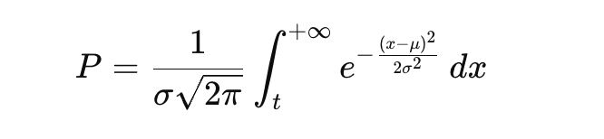
It answers:

“What is the probability that a normally distributed random variable is greater than t?”

Visualisation helps sometimes

Imagine a bell curve:

The shaded area to the right of t is exactly what this formula computes. Let’s take below example:

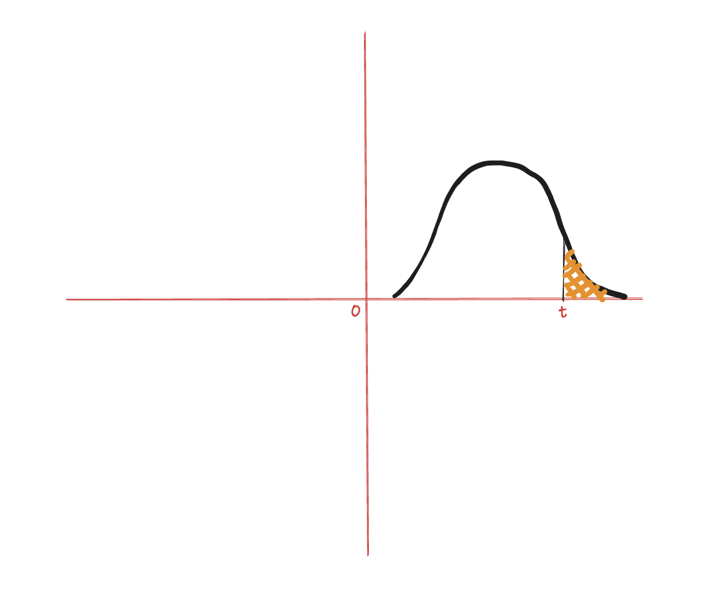
Suppose request latencies are normally distributed as,

Mean (μ) = 100 ms, Standard deviation (σ) = 20 ms

The ask: What’s the probability a request takes more than 140 ms?

Here: t = 140

The formula simply computes: P(X > 140)

Convert to Z-score

To talk in terms of standard deviation, we need to find the z-score. Look it up for more information.

A z-score (or standard score) measures exactly how many standard deviations a data point is from the dataset’s mean

First standardize:

z = (t - μ) / σ

For our example:

z = (140 - 100) / 20 = 2

Normal distribution intuition

Density decreases as we move away from the mean. The area to the right of z = 2 represents P(X > 140 ms).

On doing some integral math, the area to the right of z = 2 is about:

P(Z > 2) ≈ 0.0228 or 2.28%

Therefore by association:

P(X > 140) ≈ 0.0228 = 2.28%

Step 1: build the sample

Say you’ve collected 10 inter-arrival intervals from a peer (in seconds):

[0.95, 1.02, 0.98, 1.05, 0.99, 1.01, 0.97, 1.03, 1.00, 0.98]

μ = 1.0s    # average heartbeat gap
σ = 0.03s   # very consistent; almost never strays far from 1s

Step 2: current silence

The last heartbeat arrived 1.1 seconds ago, just 100ms beyond the mean. Suspicious?

Step 3: F(t) — the normal CDF

F(t) answers: what fraction of heartbeats from this node arrive within t seconds? In other words, how probable is it that the next heartbeat would have already arrived by now, if the node were alive?

F(t) = (1 + erf((t - μ) / (σ√2))) / 2

Short sidestep

The paper writes the tail probability as a raw integral. The problem is this integral has no closed-form solution in elementary functions.

“Elementary functions” means the basic building blocks of algebra: addition, multiplication, powers, roots, logarithms, exponentials, trig functions. A “closed-form solution” means you can express the answer using a finite combination of those.

The Gaussian integral doesn’t have that luxury. So how do we compute it then?

We approximate it numerically: pick a very small step size, slice the area under the curve into tiny rectangles, and sum them up. The more slices, the more accurate.

But doing that every time you need the value is slow. So, statisticians precomputed these values at thousands of input points, tabulated them, and gave the function a name: erf. Modern languages ship with erf as a built-in that returns these precomputed (or efficiently approximated) values instantly.

The paper’s integral form and the erf form are mathematically identical: one is the definition, the other is the computable equivalent.

So when we call erf(2.36) below, we’re not solving the integral at runtime, but looking up a highly accurate precomputed approximation.

And back

The inner term (t - μ) / (σ√2) normalises t: how many standard deviations is this silence beyond the mean? erf then maps that to a probability. Plugging in t = 1.1, μ = 1.0, σ = 0.03:

(1.1 - 1.0) / (0.03 × 1.414) = 0.1 / 0.0424 = 2.36

erf(2.36) ≈ 0.9993

F(1.1) = (1 + 0.9993) / 2 = 0.9997

99.97% of heartbeats from this node arrive within 1.1 seconds. The remaining tail ~> the probability the silence is accidental:

P(silence > 1.1s | alive) = 1 - F(1.1) = 0.0003

Step 4: φ

φ is the negative base-10 log of that tail probability:

φ = -log₁₀(0.0003) = 3.5

Just 100ms of extra silence gives φ = 3.5 on a consistent node.

Step 5: σ is doing real work

Now let’s take a jittery node: same μ = 1.0s, same 1.1s silence, but σ = 0.3s (ten times more variable):

(1.1 - 1.0) / (0.3 × 1.414) = 0.1 / 0.424 = 0.236

erf(0.236) ≈ 0.261

F(1.1) = (1 + 0.261) / 2 = 0.630

P(silence > 1.1s | alive) = 1 - 0.630 = 0.370

φ = -log₁₀(0.370) = 0.43

Same mean. Same silence. Completely different φ.

The consistent node scores 3.5 ~> suspicious. The jittery node scores 0.43 ~> totally normal.

“σ” encodes how surprising the silence is relative to that node’s own personality.

When does conviction (φ = 8) fire?

Solving backwards for each node:

Consistent node (σ = 0.03s):   conviction at t ≈ 1.24s of silence
Jittery node    (σ = 0.30s):   conviction at t ≈ 3.38s of silence

The paper is fast on well-behaved nodes and patient on variable ones, because “σ” makes the threshold adaptive per-node.

Cassandra’s simplification

Cassandra drops “σ” entirely and keeps only the mean, effectively assuming an exponential distribution (where σ = μ by definition). The formula thus collapses to:

P(silence > t | alive) ≈ e^(-t/μ)

φ = -log₁₀(e^(-t/μ))
  = (t/μ) × log₁₀(e)
  = (t/μ) × 0.4343        # PHI_FACTOR = 1/ln(10)

For the same μ = 1.0s and φ = 8 threshold:

0.4343 × (t / 1.0) = 8
t = 18.4s              # for every node, regardless of σ

–

+---------------|-------|-------------------|-----------------------+
| Node          | σ     | Paper convicts at | Cassandra convicts at |
|---------------|-------|-------------------|-----------------------|
| Consistent    | 0.03s | ~1.2s             | ~18.4s                |
| Jittery       | 0.30s | ~3.4s             | ~18.4s                |
+---------------|-------|-------------------|-----------------------+

Cassandra is far more conservative across the board. It won’t falsely convict a jittery node, but it’s also much slower to react to a dead consistent one. The trade-off: simpler implementation, no “σ” tracking, one threshold fits all node personalities.

With the same mean across two peers, Cassandra’s φ formula produces identical scores for identical silences. The consistency of the heartbeat rhythm is invisible to it.

Two nodes, both μ = 1s:

• Node A: heartbeats arrive like clockwork every 1.00s ± 0.02s
• Node B: heartbeats arrive erratically, sometimes 0.3s, sometimes 1.7s, averaging 1s

After 1.5s of silence, both get the same φ. The paper would score Node A far higher (much more suspicious) because 1.5s is wildly outside its tight σ = 0.02s window, while Node B sees 1.5s routinely.

The practical consequence in production is that we end up tuning phi_convict_threshold conservatively enough to avoid false positives on the jitteriest nodes in our cluster, which means we might be slower to convict dead consistent nodes. One threshold has to serve all node personalities because variance is invisible.

φ is not a probability at all ~> It is a score derived from one. Specifically, it is the negative log of the probability that the current silence would occur if the node were alive. The higher the φ, the less plausible the silence is from an alive node. Once you cross the threshold, you come to terms that the node might not be alive.

The sliding window

Cassandra doesn’t keep infinite heartbeat history. It maintains a bounded circular buffer of the last 1000 inter-arrival intervals per endpoint/peer ~> Check ArrayBackedBoundedStats inside FailureDetector.java.

The buffer tracks a running sum so mean = sum / count is O(1). When full, the oldest entry is evicted and the newest takes its place. The mean therefore reflects approximately the last ~1000 seconds of heartbeat history.

Two edge cases worth keeping in mind:

• Seeding: When a peer is first seen, the buffer is empty. Cassandra seeds it with a single artificial value of 2 × gossip_interval (typically 2 seconds). This gives new peers a conservatively high initial mean. They won’t be immediately suspected before the window builds up real samples.

• Window Poisoning: If a node goes through a 60-second period of elevated GC pauses, those slow inter-arrival times enter the window and inflate the mean. After recovery, the node gets more benefit of the doubt than it deserves for the next ~1000 rounds while the bad samples roll off. This is a known trade-off of the fixed-size window. To overcome this, some implementations use exponential weighted moving averages to decay old samples faster. Cassandra tends to keep it simple.

Cassandra’s implementation

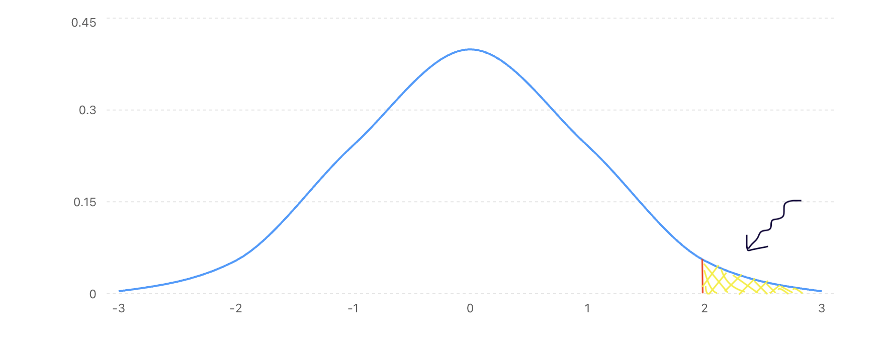
Two methods in FailureDetector.java carry the full algorithm:

report(endpoint) ~> Called every time a heartbeat arrives. Records the current nanosecond timestamp into the endpoint’s ArrivalWindow. Computing the inter-arrival interval happens inside add() on ArrayBackedBoundedStats: it subtracts tLast from now and stores that gap, then updates tLast.

// called from Gossiper.notifyFailureDetector() on every gossip state apply
ArrivalWindow heartbeatWindow = arrivalSamples.get(ep);
heartbeatWindow.add(now, ep);

interpret(endpoint) ~> Called once per gossip round (every ~1 second) from Gossiper.doStatusCheck(). Reads the window, computes φ, and if the threshold is crossed, fires conviction:

double phi = hbWnd.phi(now);   // (now - tLast) / mean

if (PHI_FACTOR * phi > getPhiConvictThreshold()) {
    for (IFailureDetectionEventListener listener : fdEvntListeners)
        listener.convict(ep, phi);
}

convict() on the Gossiper listener calls markDead(), flipping the endpoint’s isAlive flag to false. That’s what nodetool status command reads when it shows "DN" for a convicted peer.

Process control flow:

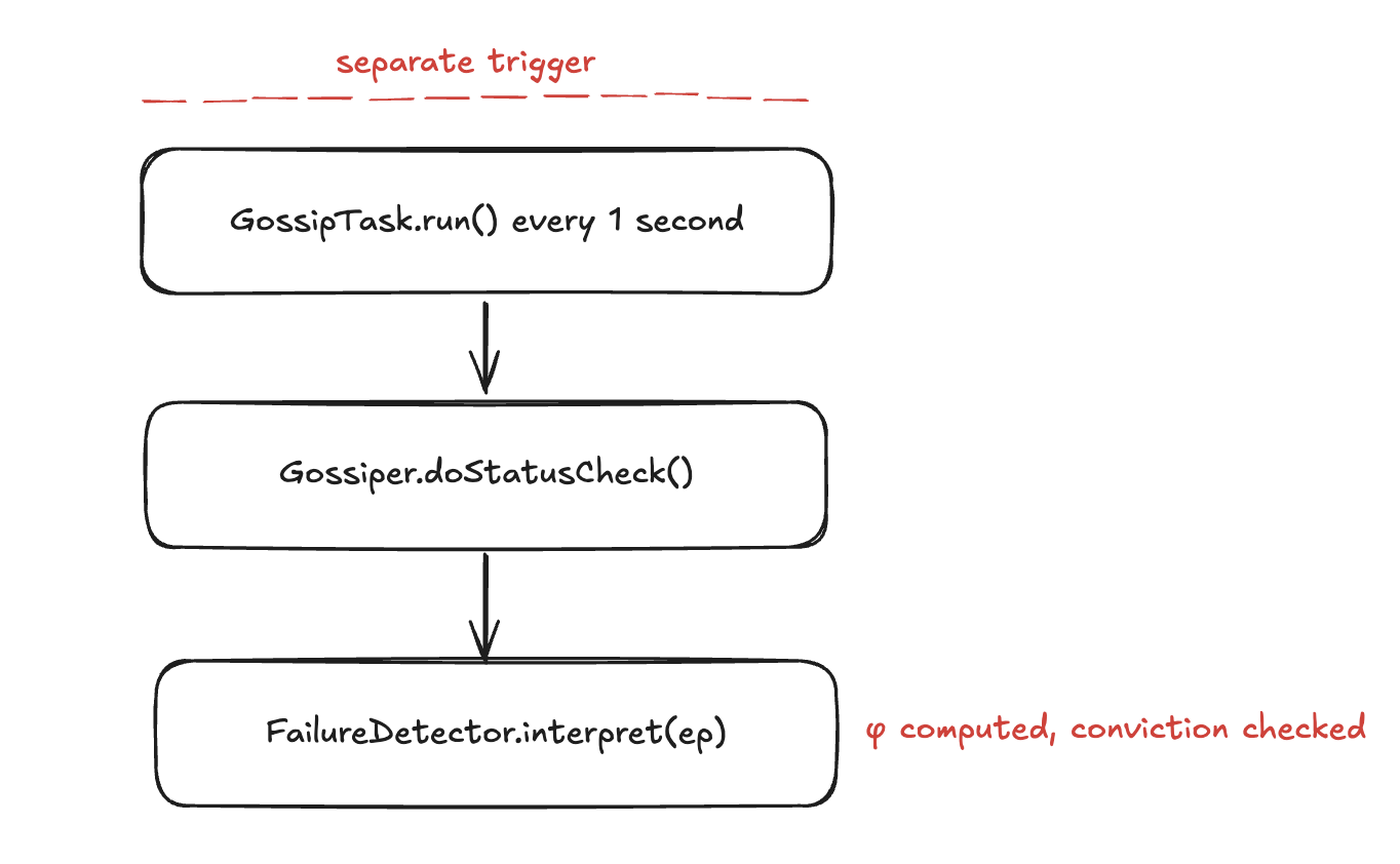
report feeds the window. interpret reads it. They bØth run on independent triggers.

PHI_FACTOR: bridging paper to code

Cassandra’s raw φ computation is just:

φ_cassandra = (now - tLast) / mean

No logarithm. A raw time ratio. This diverges from the paper’s log-probability scale. A raw value of 3.0 does not mean what φ = 3.0 means in Hayashibara’s formula.

The bridge is PHI_FACTOR:

PHI_FACTOR = 1.0 / Math.log(10.0)   // ≈ 0.4343

Applying it:

PHI_FACTOR × φ_cassandra = (1/ln(10)) × (t/μ) = (t/μ) × log₁₀(e)

This applies the paper’s φ definition (-log₁₀(probability)) but with Cassandra’s exponential approximation substituted in place of the paper’s normal distribution. They share the same structural formula but produce different numbers for the same silence duration.

The paper’s result would also factor in σ (heartbeat consistency), which Cassandra ignores. The threshold values are comparable in spirit, but not mathematically identical.

The conviction check becomes:

(1/ln(10)) × (t/μ) > 8
t/μ > 8 × ln(10)
t/μ > 18.42

Silence must be 18.42× longer than the mean for conviction to fire. At 1-second gossip interval, that’s roughly 18 seconds of silence.

The GC guard

There’s one more protection in interpret() that’s easy to miss:

long diff = now - lastInterpret;
lastInterpret = now;
if (diff > MAX_LOCAL_PAUSE_IN_NANOS) {
    logger.warn("Not marking nodes down due to local pause of {}ns", diff);
    lastPause = now;
    return;
}

lastInterpret tracks when interpret() last ran. If the gap between two consecutive calls is larger than MAX_LOCAL_PAUSE_IN_NANOS, the whole round is skipped.

Why?? If “I myself” was paused, say, my own GC ran for 3 seconds, then from my perspective every peer went silent for 3 seconds. Without the guard, I would end up convicting the entire cluster. The guard says: if I wasn’t running myself, my silence measurements are meaningless, don’t act on them.

A second condition (now - lastPause < MAX_LOCAL_PAUSE_IN_NANOS) also suppresses convictions for a cooldown window immediately after a detected pause, giving the cluster time to re-establish normal heartbeat flow.

Hands-on: watching φ climb

Mental model: This works on ANY cluster size and gives the largest divergence window (5–30 seconds). When you force-kill a node (SIGKILL), it stops sending heartbeats.

Each remaining node runs phi accrual failure detection independently. It monitors the gap between heartbeat arrivals and computes a suspicion score (φ). Each node has a slightly different heartbeat history, so they cross the suspicion threshold at different times.

No gossip round can coordinate this, each node decides on its own clock.

Set up a 4-node CCM cluster, then kill node4 hard:

In a new terminal window (T1): Install ccm first. Should be pretty standard. Just search the web on installation steps.

cd ~/path/to/source/cassandra    # I have cloned the cassandra repo
ant artifacts -Dno-checkstyle=true   # Build cassandra. Pretty standard

ccm create gossip_lab --install-dir=. -n 4 -s   # Create a 4-node cluster
ccm status

Once up, in another terminal window (T2), watch the heartbeat counter in gossipinfo on the surviving nodes:

while true; do
  echo "--- $(date +%T) ---";
  for node in node1 node2 node3; do
    state=$(ccm $node nodetool status 2>/dev/null \
              | grep "127.0.0.4" | awk '{print $1}');
    hb=$(ccm $node nodetool gossipinfo 2>/dev/null \
              | grep -A 3 "127.0.0.4" | grep "heartbeat" \
              | awk -F: '{print $2}' | tr -d ' ');
    echo "  $node sees node4: ${state:-GONE}  (heartbeat=$hb)";
  done;
  echo;
  sleep 1;
done

In initial terminal (T1): Kill node4 (no graceful shutdown, no gossip broadcast):

ccm node4 stop --not-gently   # sends SIGKILL: node4 cannot announce LEAVING

The heartbeat counter increments every gossip round while node4 is alive. The moment SIGKILL fires, it gradually freezes. What you should see (in terminal T2) is roughly:

--- 11:31:50 ---
  node1 sees node4: UN  (heartbeat=64)
  node2 sees node4: UN  (heartbeat=64)
  node3 sees node4: UN  (heartbeat=64)
  
--- 11:32:01 ---   # node4 just killed
  node1 sees node4: UN  (heartbeat=65)
  node2 sees node4: UN  (heartbeat=65)
  node3 sees node4: UN  (heartbeat=65)

--- 11:32:08 ---   # φ climbing; silence = 7s, μ ≈ 1s, φ × PHI_FACTOR ≈ 3.0
  node1 sees node4: UN  (heartbeat=65)  # counter frozen
  node2 sees node4: UN  (heartbeat=65)
  node3 sees node4: UN  (heartbeat=65)

--- 11:32:13 ---   # silence ≈ 12s, φ × PHI_FACTOR ≈ 5.2
  node1 sees node4: DN  (heartbeat=65)  # conviction fired
  node2 sees node4: DN  (heartbeat=65)
  node3 sees node4: DN  (heartbeat=65)

The frozen counter is φ climbing in slow motion. Every second that passes without a new heartbeat, (now - tLast) grows while the mean stays fixed, so φ grows linearly.

On CCM (single machine, shared kernel), all three nodes flip simultaneously because their inter-arrival histories are identical. In production, with real network jitter and independent GC pause histories per node, the three φ values diverge and nodes cross the threshold seconds apart.

That divergence window where node1 has declared node4 dead but node3 still considers it alive, is a fundamentally different problem from gossip delivery lag. Delivery lag is about news arriving late, but this is about each node making an independent probabilistic judgment at a different moment, with no mechanism to coordinate those judgments.

Conclusion

Failure detection tells each node when to mark a peer dead and can very well introduce windows where the cluster’s view is inconsistent.

If not anything, consider taking away below from this post:

• Fixed timeouts weigh between false positives and slow recovery. φ adapts to the actual heartbeat pattern of each peer, side-stepping that trade-off.
• φ is not a probability of death ~> rather it’s a derived scrore based on the probability that the current silence is normal, if the node were indeed alive. Crossing the threshold means rejecting the idea that the node is alive. So, basically give the benefit of doubt until you no longer can.
• Cassandra’s raw (t/μ) scaled by PHI_FACTOR = 1/ln(10) applies the paper’s φ definition, but under an exponential probability distribution, not the paper’s normal distribution. Cassandra ignores σ (stddev), so heartbeat consistency plays no role in conviction.
• In a real cluster each node decides independently, they can disagree on who is dead and for how long.

–

If you enjoyed reading, please “Like, Share and Subs” … Ohh wait, this ain’t YT … Adios!